読書メモ:リーダーの仮面――「いちプレーヤー」から「マネジャー」に頭を切り替える思考法
医療スタートアップでチームのマネジメントをしていることもあり、プレイヤーからマネジャーに頭を切り替える思考法というのがタイムリーすぎたので読んでみました。
250ページほどあり見た目は結構分厚いのですが、行間広めで読みやすく数時間で一気に読み切りました。
リーダーの仮面――「いちプレーヤー」から「マネジャー」に頭を切り替える思考法
リーダーの言動の重要性
プレイヤーとしてのピークは30代で年を取るごとにプレイヤー能力は低下していく。
リーダー・マネジメントスキルがないと代替可能な存在となってしまう。
よって、リーダーの言動スキルは今後重要になってくる。
良いリーダーやマネジャーのイメージとして、「リーダーの素質」や「人間性」が必要と想像してしまうが、本書ではそれらは不要と言い切っている。
リーダーに必要な考えを身に着けて頭を切り替えるための方法を教えてくれる本だ。
頭を切り替えるために
- リーダーのゴールは「チームの成果を最大化する」こと
- 感情を横に置く
- モチベーションを上げようとするのではなく、成果を出せる組織を作る
感情は上がったり下がったりするもので不安定であり、マネジメントの邪魔をするもの。
モチベーションを上げようと直接介入するよりも、成果を出せる組織を作ることで自然と良い雰囲気になりモチベーションが上がる。
頭を切り替えるための質問
プレイヤーから頭を切り替えるための質問
- いい人になろうとしていないか
- 待つことを我慢できるか
- 部下と競争していないか
- マネジメントを優先しているか
- 辞めないかを気にしていないか
リーダーがフォーカスすべき5つのポイント
以下5つのポイントに絞ってマネジメントを行うことを、本書では仮面をかぶると比喩しています。
- ルール
- 位置
- 利益
- 結果
- 成長
これはいわば成果を出すために立ち返るリーダーの軸であり、
常にこのポイントに立ち返って考えることを推奨している。
ルール
全員が守れるルールを言語化して、守らせること
自由度が高すぎてもストレスになる。適切なルールを設定することが重要。
ルールには2種類ある
- 行動ルール
- チームの目標に連動したルール
- 姿勢ルール
- だれでもできるもの(あいさつをしましょう 5分前行動)
ルールを設定する際の注意点として、「誰がいつまでに何をやるか」を明確にすることが重要。より具体的にルールを決めておくこと。
位置
組織内で自分がどの位置にいるのかを把握し、適切なコミュニケーションをとること
言い換えると「視座を上げる」という言葉がしっくりくる。
組織内での自分の位置を把握し、意思決定の範囲を考える。例えば、部下から言われたことをそのまま上司に伝えたりする伝言ゲームをしているような人は自分の意思決定の範囲がわかっていない。
プレイヤーの視点ではなく、少し高い位置にいることを意識することで頭を切り替える。
■位置関係を意識した指示の出し方
- 言い切り
- 締め切りの提示
- 報告するように指示
例:「〇〇してください。17時までに報告してください」
指示は上から下、報告は下から上
■報連相で相談に乗ってよいこと
- 部下の権限では決められないこと
- 部下が自分で決めていい範囲なのか迷ったとき
必要以上に相談に乗ると、部下の責任範囲を狭くして言い訳できる環境を作ってしまう。
利益
集団の利益から個人の利益が生まれる。
会社に使われる人がうまく成長できる。
集団として利益を上げることで、個人は利益を得ることができる。
結果
プロセスではなく結果をみる。
未来への視点を持つ。
結果を管理すること。目標設定をして仕事を任せ、結果を報告してもらい評価する。
■点と点の目標設定
- 目標設定 → 数値化、言い切る、締め切り
- プロセス → 口出ししない
- 結果 → 事実だけの報告をさせる
- 未達の場合
- できてなかったことを指摘
- 具体的な行動を考えさせる
- 「次はどうしますか?」
- 1つ前のプロセスを目標に加える(成約数が未達成の場合、訪問数を目標に追加)
- 達成の場合
- 結果だけを受け取る
- 未達の場合
- 次の目標を具体帝に言語化
成長
経験とともにしか人は成長できない
まずは部下に経験させることが大事。
まとめ
本書のように自分なりの「軸」を持つことでブレないマネジメントができそうなので試してみたいと思った。
内容を機械的にマネするだけでは使い物にならないので、自らのパーソナリティや状況によって段階的にエッセンスを取り入れていくのがよさそう。
カレンダーライブラリFullCalendarをReactでカスタマイズして使う
GoogleカレンダーのようなカレンダーUIを簡単に作れるライブラリ「FullCalendar」を実務で使う機会があり、色々とカスタマイズして使ってみたので整理しておく。
「最もポピュラーなJavaScriptカレンダー」
カレンダーライブラリの選定
カレンダーライブラリを使うにあたり調査しました。候補としては以下の2つ。
どちらも同じようなAPIが用意されており、共通で以下の特徴がありました。
-
TypeScript対応
-
メンテナンスが盛ん
-
日本語対応
-
ドキュメントが豊富
-
セル内のカスタマイズ自由度→どちらもコンポーネントをPropsとして渡せる
FullCalendarの方が日本語対応が簡単で、開発速度出せそうな感じがしたので採用。
React用のラッパーライブラリを別途インストールする必要があります。
FullCalendarのカスタマイズ
ほぼドキュメントに載っているため、ドキュメント読めばわかるといえばそれまでなのですが、せっかくなのでカスタマイズした内容をメモっておきたいです。
基本のカレンダー
locale、timeZoneを指定するだけで日本対応が可能です。
あとはカレンダーに表示するイベントデータ events と読み込んだプラグインを渡すだけです。
プラグインは、timeGridなど様々なものが用意されていますので用途によって選択します。ここでは、dayGridの通常のカレンダーとインタラクションを与えるプラグインを読み込んでいます。
import FullCalendar from '@fullcalendar/react'
import dayGridPlugin from '@fullcalendar/daygrid'
import interactionPlugin from '@fullcalendar/interaction'

<FullCalendar
  locale='ja'
  timeZone='Asia/Tokyo'
  events={eventData}
  plugins={[dayGridPlugin, interactionPlugin]}
/>
カレンダーに表示するイベントデータ
カレンダーにイベント情報を表示させるには、FullCalendarで定義されているイベントオブジェクトの形式に則る必要があります。
events: [
  {
    title: 'BCH237',
    start: '2019-08-12T10:30:00',
    end: '2019-08-12T11:30:00',
    extendedProps: {
      department: 'BioChemistry'
    },
    description: 'Lecture'
  }
  // more events ...
],
Event Objectとして定義されていて、このオブジェクトの形式に合わせて整形してprops events へ渡します。
プロダクト独自の項目をもたせたい場合は、 extendedProps に格納すれば対応できます。
デフォルトのヘッダーを独自のコンポーネントにカスタマイズする
カレンダーの上部にはデフォルトで「今日」ボタン、翌月、前月ボタンなどのインタラクションが用意されています。
そのままだとイケてないので、独自のコンポーネントでカスタマイズしたい場合が多いかと思います。
CalendarAPIを利用することで、本日の日付に移動したり、翌月に移動させたりすることが可能です。
import FullCalendar from '@fullcalendar/react'

// useRefを使ってインスタンス化する
const calendarRef = useRef<FullCalendar>(null)

// calendarRefのgetApi()でメソッドを呼び出す
const goToNext = () => {
  if (calendarRef.current) {
    calendarRef.current.getApi().next()
    setCurrentDate(calendarRef.current.getApi().getDate())
  }
}

// calendarRefのgetApi()でメソッドを呼び出す
const goToPrev = () => {
  if (calendarRef.current) {
    calendarRef.current.getApi().prev()
    setCurrentDate(calendarRef.current.getApi().getDate())
  }
}

// calendarRefのgetApi()でメソッドを呼び出す
const goToToday = () => {
  if (calendarRef.current) {
    calendarRef.current.getApi().today()
    setCurrentDate(calendarRef.current.getApi().getDate())
  }
}

// ....

// 独自のコンポーネント
<Button onClick={goToToday}>
  今日
</Button>
<Button onClick={goToPrev}>
  前月
</Button>
<Button onClick={goToNext}>
  来月
</Button>
<FullCalendar
  locale='ja'
  timeZone='Asia/Tokyo'
  events={eventData}
  plugins={[dayGridPlugin, interactionPlugin]}
	ref={calendarRef} // RefObjectを渡す
/>
こうすることで、ヘッダー部分のボタン群を独自のコンポーネントへ置き換えることができます。
各種Props
FullCalendarには様々な設定が用意されており、かなり柔軟に対応できるかと思っています。
ただし、一部UIがイケてなかったり、挙動が微妙なものもあるので、その場合は独自コンポーネントに置き換えたりする必要があるかと思っています。
-
eventClick:イベントクリック時にイベント情報を持つEventClickArgを受け取れます。イベント情報の詳細を確認したいときや編集画面を表示させたい時に使えます。
-
fixedWeekCount:これをfalseにしていないと、固定で第5周目まで表示され、第5週目が無い月は、翌月の月初の日付が表示されてしまうので、かなり無駄が多かったです。
-
dayMaxEvents:1日のイベント数の表示上限を設定できます
-
moreLinkContent:上記dayMaxEventsの数を超えた場合、
more +3といった文字列が表示されます。このコールバック関数に表示したい文字列を渡してカスタマイズできます。 -
dayCellContent:カレンダーの各日の日付部分の表記を変更できます。日本語対応だと「5日」みたいに必ず’日’が入ってくるのが邪魔な場合はここでreplaceしてあげると解決します。
-
eventContent:イベント情報を持つEventContentArgを受け取り、JSXを返す関数を渡せば、カレンダー上に表示させるイベント情報をカスタマイズできます。
-
dayPopoverFormat:morelinkをクリックした時に表示されるPopoverの日付フォーマットを指定できます。
-
headerToolbar:デフォルトのヘッダーツールバーを非表示にできます。ツールバーをカスタマイズしたかったので
falseに設定しました。
カスタマイズに関して、日本語情報が少ない
この他にも色々とカスタマイズしていますが、日本語情報が少なく、特にReactを使った実装方法が少ないと感じました。
もともとFullCalendarはReact専用ライブラリではなく、JavaScriptライブラリなのでjQueryを使った記事が多かったです。
あとはバージョンの違いでAPIが廃止されてたり、かなり破壊的なバージョンアップが行われている印象を受けました。
ドキュメントを読み溶けるのであれば困らないかもしれませんが、個人的は微妙に苦戦しました。
参考リンク
https://www.mitsue.co.jp/knowledge/blog/frontend/202012/08_0900.html
styled-componentsでcss propsを使うために苦戦した話
やりたいこと
styled-componentsでcss propsを使ってスタイリングをしたい
開発環境
開発環境はCRAで構築したReactアプリケーションであり、TypeScript、styled-componentsを採用している。 コンポーネントへのスタイル注入方法を検討中、css propsを活用したかった。
-
typescript ... 4.6.3
-
react ... 18.0.0
-
styled-components ... 5.3.5
結論を先に述べると、以下の設定が必須であった。
-
css propsの型定義
-
Babel macrosのインポート
エラー内容
import React from 'react'
import { css } from 'styled-components'

const styles = {
  text: css`
  font-size: 32px;
  color: red;
`,
}

// DOM component
export const StylingTest: React.FC = (props) => {

  return (
    <div>
      <p css={styles.text}>Dashboard</p> // error!!
    </div>
  )
}
型 '{ children: string; css: FlattenSimpleInterpolation; }' を型 'DetailedHTMLProps<HTMLAttributes<HTMLParagraphElement>, HTMLParagraphElement>' に割り当てることはできません。 プロパティ 'css' は型 'DetailedHTMLProps<HTMLAttributes<HTMLParagraphElement>, HTMLParagraphElement>' に存在しません。 ts(2322)
TypeScriptエラーが出た。 styled-componentsの場合、css propsを利用するのにcssの型を定義する必要がある?と思ったが、 jsxファイルにして試した見たところ、スタイリングが反映されない。
つまり、TypeScriptの型定義設定と、Styled-componentsライブラリの設定それぞれが必要だと推察した。
「styled-components css props typescript」でググる
styled-components: API Reference
To enable support for the css prop you have to use the Babel plugin.
babel pluginとやらを使用する必要があるみたいだ。
Babel macros are quickly gaining steam as a full-featured option to allow advanced code transpilation for zero-config projects like create-react-app. If your scaffold is set up with babel-plugin-macros, then simply use the new styled-components/macro import instead of styled-components:
create-react-appなどで構築したアプリケーションには、babel macrosを使えば良いと書いてある。 babel-plugin-macros,が設定されている必要があるみたいだが、create-react-appには既にbabel-plugin-macrosが導入されているみたいなので、別に設定は不要だと解釈した。
ここまでで、CSS Propsの章へ戻る。
Usage with the Babel macro You can use the Babel macro to make this work in create-react-app. Unfortunately, Babel macros only run when imported so the import can not be added automatically. The above code works perfectly if you add the import to the macro manually: Babel macros only run when imported so the import can not be added automatically
とあり、create-react-appで作成したプロジェクトについてはbabelで自動インポートがされず、手動でインポートが必要と書かれている。
TypeScript対応の箇所を見ると、declare moduleで定義 或いは 以下のインポートが必要と書かれている
import {} from 'styled-components/cssprop'
こちらのissueを見てみると index.d.ts に以下の記述があるらしい
/**
 * The CSS prop is not declared by default in the types as it would cause 'css' to be present
 * on the types of anything that uses styled-components indirectly, even if they do not use the
 * babel plugin.
 *
 * You can load a default declaration by using writing this special import from
 * a typescript file. This module does not exist in reality, which is why the {} is important:
 *
 * ```ts
 * import {} from 'styled-components/cssprop'
 * ```
 *
 * Or you can declare your own module augmentation, which allows you to specify the type of Theme:
 *
 * ```ts
 * import { CSSProp } from 'styled-components'
 *
 * interface MyTheme {}
 *
 * declare module 'react' {
 *   interface Attributes {
 *     css?: CSSProp<MyTheme>
 *   }
 * }
 * ```
 */
styled componentsのcss prop - Qiita
babel-plugin-styled-components を使用する必要があるとここでも書かれている。 PullRequestが解決されれば、DefinitelyTyped側に反映されるはずだが、まだOpenになっているし、まだ反映されていないのか??
styled-componentsのcss propsが動作しないという投稿。V4系からcss propsが登場したが、まだ不具合が多いっぽい??
原因
-
css props機能を有効にするには,
babel-plugin-styled-componentsを使用する必要があった -
create-react-appで作成したプロジェクトではBabel macrosを手動でインポートが必要だった
-
まだDefinitelyTypedに反映されておらず、CssPropsの型定義をインポートする必要があった
コード例
styled-components.d.tsをプロジェクト内に作成
import { AppTheme, MuiTheme } from 'styles/theme'
import { CSSProp } from 'styled-components'

declare module 'styled-components' {
  interface DefaultTheme extends MuiTheme {}
}

declare module 'react' {
  interface Attributes {
    css?: CSSProp<MuiTheme>
  }
}
import React from 'react'
import { css } from 'styled-components/macro'

const styles = {
  text: css`
  font-size: 32px;
  color: red;
`,
}

// DOM component
export const StylingTest: React.FC = (props) => {

  return (
    <div>
      <p css={styles.text}>Dashboard</p>
    </div>
  )
}
styled-components/macro を呼び出さないとcss propsでスタイルが反映されなかった。 styles の定義を別ファイルで切り出す場合、 styled-components/macro をコンポーネント側でインポートしないとCSSが反映されなかった。 App.tsx などで呼び出せばすべてのコンポーネントで反映されるか?と思いきやそれもだめ。css props を使用するコンポーネントでBabel macrosを手動でインポートしないと動作しないことがわかった。
以下のようなイメージ。
import React from 'react'
import 'styled-components/macro'

import { styles } from './styles'

export const StylingTest: React.FC = (props) => {

  return (
    <div>
      <p css={styles.text}>Dashboard</p>
    </div>
  )
}感想は、めちゃくちゃ苦戦した。styled-componentsでcss propsを使うのは一筋縄じゃいかないので、素直にemotionとかを使った方が良さそうだなと感じた。
参考リンク
JavaScriptの配列操作についての整理
JavaScriptでの配列操作を使う機会が多いが、毎回ググってる気がするのでひとまずよく使うものについて整理してみる。
配列操作
  const arr1 = [10, 20, 30];
  const arr2 = [40, 50, 60];

  const arrObj = [
    {
      id: 1,
      name: "A"
    },
    {
      id: 2,
      name: "B"
    },
    {
      id: 3,
      name: "C"
    },
    {
      id: 4,
      name: "D"
    },
    {
      id: 5,
      name: "E"
    },
    {
      id: 6,
      name: "F"
    }
  ];
length
配列の要素数を取得する 返り値:number
  const arr1 = [10, 20, 30];

  console.log("length", arr1.length);
  // => length 3
indexOf
見つかった最初の要素の添字を返す、見つからなかった場合は-1を返す 返り値:number
  const arr1 = [10, 20, 30];

  console.log("indexOf", arr1.indexOf(20));
  // => indexOf 1
  console.log("indexOf", arr1.indexOf(40));
  // => indexOf -1
join
全要素を順に連結した文字列を新たに作成 区切り文字を指定できる 返り値:string
  const arr1 = [10, 20, 30];

  console.log("join", arr1.join());
  // => join 10,20,30
slice
配列のすべてまたは一部をコピーする 返り値:Array
  const arr1 = [10, 20, 30];

  console.log("slice", arr1.slice(2));
  // => slice [30]
concat
配列同士を結合 返り値:Array
  const arr1 = [10, 20, 30];
  const arr2 = [40, 50, 60];

  console.log("concat", arr1.concat(arr2));
  // => concat [10, 20, 30, 40, 50, 60]
reverse
逆順 返り値:Array
  const arr1 = [10, 20, 30];

  console.log("reverse", arr1.reverse());
  // => reverse [30, 20, 10]
sort
並び替え 返り値:Array
  const arr1 = [10, 20, 30];

  console.log("sort", arr1.sort()); // 昇順
  console.log(
    "sort",
    arr1.sort((x, y) => y - x)
  ); // 降順
  // => sort [30, 20, 10]
map
新しい配列を生成 全ての要素に対して関数を一度ずつ実行,新しい配列を生成 返り値:Array
  console.log(
    "map",
    arrObj.map((item) => ({ id: item.id + "_map", name: item.name + "_map" }))
  );
  // => map [{id: "1_map",name: "A_map"} ...]
filter
絞り込み(複数要素) true を返した要素からなる新しい配列を生成 返り値:Array
  console.log(
    "filter",
    arrObj.filter((item) => item.id % 2 === 0)
  );
  // filter [{id:2, name: "A"},{id:4, name: "D"},{id:6, name: "F"}]
find
絞り込み(1要素) true を返す要素が見つかるまで、要素に対して一度ずつ関数を実行する 返り値: Arrayの1要素
  console.log(
    "find",
    arrObj.find((item) => item.id === 5)
  );
  // => find {id: 5, name: "E"}
some
true を返す要素が見つかるまで、要素に対して一度ずつ関数を実行,1つでもtrue を返す要素が見つかると、 true を返す。 返り値: boolean
  console.log(
    "some",
    arrObj.some((item) => item.id === 5)
  );
  // => some true
every
false を返す要素が見つかるまで、要素に対して一度ずつ関数を実行,false を返す要素が見つかると、 false を返す。すべてがtrueであればtrueを返す 返り値: boolean
  console.log(
    "every",
    arrObj.every((item) => item.id !== null)
  );
  // every false
reduce
配列を繰り返し処理し、計算結果を返す 返り値:計算結果
  console.log(
    "reduce",
    arr1.reduce((prev, current, index) => prev + current)
  );
TypeScriptでundefined or nullを真偽値に変換する
やりたいこと
null や undefined の値をfalsyな真偽値として扱いたい
結論
Boolean() あるいは !!で二重否定を使う。
  const unData = undefined;
  const nullData = null;
  const strData = "";
  const arrData: string[] = [];
  const objData = {};

      // !! をつけることで、 nullの場合、undefinedの場合にfalseとなる

    // false
    console.log("unData", !!unData);

    // false
    console.log("nullData", !!nullData);

    // 空文字列もfalseになる
    console.log("strData", !!strData);

    // 空配列はtrueになる
    console.log("arrData", !!arrData);

    // オブジェクトはtrueになる
    console.log("objData", !!objData);
単純に nullの場合はnull。!nullとした場合はnullの否定なのでtrue。 !!nullとした場合は二重否定となるのでfalseとなる。
undefined や 空文字列('') でも同じ挙動を確認できた。 空配列やオブジェクトに対しては使えない。
Reactで和暦と西暦の表示切り替えをする関数を書いた
すでに令和も4年。平成まではギリ西暦⇔和暦の変換ができていたけれど、令和になってからは覚えるのもめんどくさくなり、ググらないと今は令和何年なのかもわからないという人もいるのでは?
前職は病院の事務員だったので、様々な行政の書類や日々の業務の中で和暦にふれる機会が多かったのですが、、IT業界へ転職し、書類を処理したり患者様の対応をすることもないので、わざわざ和暦で年を数えることもなくなりました。
ただし、役所や医療機関など行政書類を扱ったり、保険情報などを扱う場合は和暦が標準になっているケースが多く、そういった業務アプリの開発には和暦対応も要求されると思っています。
今回は、和暦⇔西暦で相互変換する関数を実装してみました。
やりたいこと
やりたいことをざっと書き出してみたのが以下
-
和暦⇔西暦の切り替えボタンにより、表示形式の切り替えができる
-
ページ内に存在する日付データの形式がまとめて切り替わる
-
あくまで表示を切り替えるだけで元データには影響を与えない
実装イメージ
-
親コンポーネント(Page)でboolean型の表示形式の状態を持つ
-
親コンポーネント(Page)でstring型の日付データを持つ。
-
日付データは必須項目である
-
関数は日付情報と表示形式の状態を引数として受け取る
-
表示形式の状態によって、和暦と西暦の表示切り替えをする
結論
まずは結論として、Codesandboxを御覧ください。
https://codesandbox.io/embed/date-he-li-xi-li-og86ng?fontsize=14&hidenavigation=1&theme=dark
表示切り替えのボタンをクリックすると、BirthDayの一覧すべての項目に対し、表示形式の切り替えができます。
メインとなるのは utils.ts に定義している関数 conversionBetweenJpAndAdです。
dummy.ts は単なるダミーデータなので割愛。
実装方法
utils.ts
import { parse } from "date-fns";
import ja from "date-fns/locale/ja";

export const conversionBetweenJpAndAd = (date: string, jpFormat: boolean) => {
  if (jpFormat) {
    const jp = new Intl.DateTimeFormat("ja-JP-u-ca-japanese", {
      era: "long",
      year: "numeric",
      month: "long",
      day: "numeric"
    }).format(
      new Date(parse(date, "yyyy年M月d日", new Date(), { locale: ja }))
    );

    return jp;
  }

  return date;
};
日付ライブラリは date-fnsを使いました。
date-fnsは日付データのパースに使用している程度で、本命は Intl.DateTimeFormatです。
Intlは国際化APIの名前空間で、数値フォーマットや表示名の翻訳など国ごとの表記に変換するAPIが用意されています。
その中の一つが今回使用したIntl.DateTimeFormat()で、言語に依存した日時のフォーマットができるAPIです。
Intl オブジェクトは、 ECMAScript の国際化 API の名前空間で、言語に依存した文字列の比較、数値の書式化と、日付の書式化を提供します。 Intl オブジェクトは、いくつかのコンストラクターに加え、国際化コンストラクターや他の言語に関する関数に共通する機能へのアクセスを提供します。
-
第一引数 ... locale(日本であればja-JP-u-ca-japanese)
-
第二引数 ... options(年、月、日の表記形式やタイムゾーンの表記形式など)
第二引数にeraを指定すると、元号を付与して表示させることができます。
今回はstring形式の日付データを扱うため、フォーマットする際は、string形式の日付データをdate-fnsでDate型にパースして渡してあげる必要があります。
あとは、表示形式の状態を定義したjpFormatを受け取って条件分岐させ、jpFormatでない場合は日付データをそのままreturnするようにしました。
親コンポーネントApp.tsx
親コンポーネント側では、jpFormatとして表示形式の状態をboolean型で定義し、Buttonをクリックした際にstateを更新するようにします。これによって、和暦⇔西暦の切り替えを実現させます。
usersデータを表示させる際、conversionBetweenJpAndAdを呼び出してuser.birthDateとjpFormatを引数として渡してあげれば完成です。
App.tsx
import { useState, useCallback } from "react";
import { conversionBetweenJpAndAd } from "./utils";
import { users } from "./dummy";
import "./styles.css";

export default function App() {

  const [jpFormat, setJpFormat] = useState<boolean>(false);
  const onChangeDateViewType = useCallback(() => {
    setJpFormat((prevState) => !prevState);
  }, []);

  return (
    <div className="App">
      <div className="button">
        <button onClick={onChangeDateViewType} type="button">
          {jpFormat ? "西暦表示" : "和暦表示"}
        </button>
      </div>
      <ul className="list">
        <li className="listHead">
          <span>ID</span>
          <span>UserName</span>
          <span>BirthDay</span>
        </li>
        {users.map((user) => (
          <li key={user.id}>
            <span>{user.id}</span>
            <span>{user.name}</span>
            <span>{conversionBetweenJpAndAd(user.birthDate, jpFormat)}</span>
          </li>
        ))}
      </ul>
    </div>
  );
}
所感
和暦って、正規表現で処理マッチさせて処理を書いていくイメージだったのですが、Intl.DateTimeFormatとdate-fnsを使うことで簡単に実装できました。
ググっても和暦⇔西暦の切り替え機能を作っている人はあまりいなく、こういった実装方法で問題がないのかは不安ではありますが、イメージどおりの動きをしてくれていると思います。
「平成6年って、西暦何年だっけ?」みたいなケースにサクッと切り替えられるのは個人的には嬉しい。使える機会があれば業務アプリの開発で使ってみようと思います。
参考リンク
E2EテストにCypressを導入する
E2Eテストとは何か?
End to Endテストの略であり、ユーザー利用と同じようにシステム全体を操作して確認するテストのこと
テストを自動化するメリデメ
-
メリット
-
反復的な手作業のコストを削減できる
-
テストの実施コストが下がり、早期にバグチェックがしやすい
-
同じ手順で同じテストを行うため、再現性が高い
-
品質がテスト実行者の習熟度に左右されない
-
-
デメリット
-
テストツールの使い方を学ぶ必要がある
-
自動テストのメンテナンスコストがかかる
-
運用体制が整っていないと無駄になる場合がある
-
テスト自動化はかならずしも品質向上、コスト削減が実現するものではない。
E2Eはシステムの細かな修正1つで壊れることが多く、メンテナンスが大変
Cypressの特徴
-
非同期処理に強い
-
対象のDOMが見つかるまで一定時間単柵を行う
-
アクションが実行された時点でDOMが存在しない場合でもタイムアウトまでにDOMが描画されれば、エラーにならずテストが継続できる
-
待機処理やレスポンスが帰るまでリトライする処理を必要としない
-
-
環境設定が簡単
-
ブラウザやドライバをインストールする必要がない
-
スクリーンショットやビデオ出力、、タイムトラベルなどデバッグを手助けする機能が備わっている
Cypressでテストを構築
install
yarn add cypress
管理画面の起動
npx cypress open
管理画面を起動すると、自動的に /cypress ディレクトリ配下に自動で構成される。
./
├──cypress
│  ├──fixtures
│  ├──integration
│  ├──plugins
│  └──support
├──node_modules
├──cypress.json
└──packagelock.json
-
cypress/fixtures-
テストで扱う静的データ
-
fixtures配下のファイルはテストコードの中で読み込んで使用できる
-
-
cypress/integration-
テストコードを記述したファイルを
integration配下に置くことで実行ファイルとして認識される
-
-
cypress/plugins-
Cypressの裏側で実行されるNode.jsの処理ファイル
-
テストの前後処理やプラグインの構成を記述する
-
-
cypress/support-
Cypressテストを補助する処理ファイル置き場
-
support配下のファイルはテスト実行時に1度だけ実行される
-
-
cypress.json-
環境設定やタイムアウトの設定など
-
Cypressでテストを書く方法
describe() を使って、一定の単位でテストを宣言
その中で it() を使ってテストの詳細を書いていく
describe('機能A', () => {
	it('正常値入力の確認', () => {
		// テスト内容
	})
	it('異常値入力の確認', () => {
		// テスト内容
	})
}
Webサイトへアクセス: visit()
遷移先URLを指定し、ブラウザを指定のURLにアクセスさせる。
cypress.json で baseUrlが定義されていたら、 baseUrl からの相対パスを指定する。
cy.visit('<https://www.google.com/>')
cy.visit('./login')
操作したいDOMを取得: get() , contains()
指定のDOMを取得するコマンド
-
get() -
contains()-
DOMが包含する文字列かセレクタを指定してDOMを取得
-
文字列などで簡単に取得できる一方で、メッセージの変更でテストが壊れやすいので注意
-
cy.get('.submitButton')
cy.contains('送信')
DOMにアクションを加える: click() , type()
-
click()-
クリック操作
-
-
type()-
キーボード入力
-
cy.contains('送信').click()
cy.get('input').type('山田太郎')
アサーション: should()
BDD、TDDの概念に基づくアサーションコマンド
-
should()-
宣言した内容が正しいかどうかを判定してアラートを出す
-
cy.contains('山田太郎').should('exist')
cy.get('submitButton').should('be.disabled')
テストの前後処理: beforeEach() , afterEach() , before(), after()
-
beforeEach() -
afterEach()itで宣言されたそれぞれのテストに対して、前処理や後処理を定義できる
ログイン処理など、テストに共通する処理をまとめて記述する際に便利
-
before() -
after()describe()で定義されたテスト単位の中で一度だけ実行される前後処理テスト対象であるシステムのデータ更新に便利
describe('機能A', () => {
	before(() => {
		// 最初に一度だけ実行したい前処理を記述
	})

	beforeEach(() => {
		// 各テストに共通する前処理
	})

	it('正常値入力の確認', () => {
		// テスト内容
	})
}
特定のテストのみ実行する: only()
任意のテストのみ実行させるコマンド
開発中のテストコード部分のみテストしたい場合など
describe('機能A', () => {
	it.only('正常値入力の確認', () => {
		// テスト内容
	})

	//実行されない↓

	it('異常値入力の確認', () => {
		// テスト内容
	})
}
特定のテストの実行をスキップ: skip() , xit()
特定のテストをスキップできる
describe('機能A', () => {

	//実行されない
	it.skip('正常値入力の確認', () => {
		// テスト内容
	})

	//実行されない
	xit('異常値入力の確認', () => {
		// テスト内容
	})
}
簡単なログイン機能をテストする
describe('ログイン機能', () => {
  beforeEach(() => {
    cy.visit('<http://localhost:3000>')
  })

  it('正常値入力の確認', () => {
    cy.get('.inputName').type('山田太郎')
    cy.get('.inputPassword').type('yamadaPass1234')
    cy.get('.button').click()
    cy.contains('成功しました').should('exist')
  })
})
GUIを使ったテスト
npx cypress open
CLIを使ったテスト
npx cypress run
ToDoアプリのテスト
// 関数として定義して使い回す
const addTodo = (value) => {
  // valueを入力してenterキーを発火させる
  cy.get('.new-todo')
    .type(value)
    .should('have.value', value)
    .type('{enter}', { delay: 100 })
  // 入力欄に値が無いことを確認する
  cy.get('.new-todo').should('have.value', '')
  // コンテンツがレンダリングされていることを確認する
  cy.contains(value)
}

const deleteTodo = (nth) => {
  // .invoke('show') でホバーコンテンツを表示させてクリック
  cy.get(`.todo-list > li:nth(${nth}) .destroy`).invoke('show').click()
}

describe('ToDoアプリ', () => {
  beforeEach(() => {
    cy.visit('<https://example.cypress.io/todo>')
  })

  it('add 3 todo and delete middle todo', () => {
    addTodo('todo1')
    addTodo('todo2')
    addTodo('todo3')
    deleteTodo(3) // 2つ目を削除
  })
})
CustomCommandsでコマンドを使い回す
複数のspecファイルで使用する可能性がある場合、CustomCommandsで定義する
時分のほしいコマンドを cy.contains や cy.get と同じように作成できる
cypress/support/commands.js
//  cy.addTodoとして呼び出せる
Cypress.Commands.add('addTodo', (value) => {
  cy.get('.new-todo')
    .type(value)
    .should('have.value', value)
    .type('{enter}', { delay: 100 })
  // 入力欄に値が無いことを確認する
  cy.get('.new-todo').should('have.value', '')
  // コンテンツがレンダリングされていることを確認する
  cy.contains(value)
})

//  cy.deleteTodoとして呼び出せる
Cypress.Commands.add('deleteTodo', (nth) => {
  cy.get(`.todo-list > li:nth(${nth}) .destroy`).invoke('show').click()
})
Jestとの使い分け
Cypressのメリット
-
Cypress固有の自動リトライにより、ウェイト処理といった低水準な処理が少ない高水準なテストが書ける
-
失敗時に「こういうロールはあるがこれはなかった」といったエラーが出るのがわかりやすい。それぞれのステップのDOMツリーを見ながらデバッグできる
-
完成品のWeb画面へのテスト、とくに画面遷移を含んだテストがやりやるい
Jestのメリット
-
圧倒的に高速
-
ReactHooksのテストなど、テスト用カスタムコンポーネントを作るのが楽
Jestでユニットテストを書いてカバレッジを上げつつ、Cypressを使っていくのがいい。
cypressテスト用リポジトリ
create-react-appで生成されるmanifest.jsonとは何か
create-react-app で生成されている /public/manifest.json とは何者なのか?無知であったマニフェストファイルについて改めて調べてみた。
調査前の前提知識
デフォルトで生成される manifest.json
{
  "short_name": "React App",
  "name": "Create React App Sample",
  "icons": [
    {
      "src": "favicon.ico",
      "sizes": "64x64 32x32 24x24 16x16",
      "type": "image/x-icon"
    },
    {
      "src": "logo192.png",
      "type": "image/png",
      "sizes": "192x192"
    },
    {
      "src": "logo512.png",
      "type": "image/png",
      "sizes": "512x512"
    }
  ],
  "start_url": ".",
  "display": "standalone",
  "theme_color": "#000000",
  "background_color": "#ffffff"
}
見た感じ、ファビコンなどのアイコンがセットされているので、Webサイト公開に必要なアイコンセットを定義できるもの?という認識
start_url や display: standalone など用途不明なものがおおい。
マニフェストファイルとは
manifest.json は、マニフェストファイルと呼ばれるもので、プログレッシブウェブアプリ (PWA)の振る舞いを設定するJSONファイル。
プログレッシブウェブアプリ (Progressive web apps, PWA) は、新しいウェブ API と伝統的なプログレッシブな拡張戦略を使用して、クロスプラットフォームのウェブアプリケーションにネイティブアプリと同様の使い勝手をもたらすウェブアプリのこと
既存のサイトをPWAにするには、以下の手順が必要。
-
HTTPSに対応する -
manifest.jsonを設置する -
Service Workerを有効にする
Service Workerを有効にしていなくても、スマホでホーム画面にWebアプリを追加できるA2HS という機能はデフォルトで使用できる。 その際の振る舞い、アイコンの設定ができる。
htmlファイルへはmanifestとして読み込ませると適用される
<link rel="manifest" href="/manifest.json" crossorigin="use-credentials">
マニフェストファイルのプロパティ
-
short_nameおよび/またはname(必須) ... 少なくともshort_nameまたはnameプロパティを提供する必要がある。両方が提供short_nameされている場合は、ユーザーのホーム画面、ランチャー、またはスペースが限られている可能性があるその他の場所で使用されます。nameアプリのインストール時に使用されます。 -
icons... PWAをインストールすると、ホーム画面、アプリランチャー、タスクスイッチャー、スプラッシュ画面などで仕様するアイコンを定義できる。SVGも対応しているっぽいが、アイコンがインストール時のままになってしまう。 -
start_url(必須) ... 起動時にアプリケーションを起動する場所を指示できる。ユーザーがアプリをホーム画面に追加したときに表示されていたページからアプリが毎回起動しないようにする。 -
background_color... アプリがモバイルで最初に起動されたとき、スプラッシュ画面で使用される -
display... アプリの起動時に表示されるブラウザーUIをカスタマイズできる -
fullscreen... ブラウザUIなしでアプリケーションを開き、使用可能な表示領域全体を占有 -
standalone... スタンドアロンアプリ風に開く。ブラウザとは別の独自ウィンドウで実行され、URLなどの標準のブラウザUI要素が非表示になる -
minimal-ui... スタンドアロンに加えて戻る、リロードなどのセットをユーザーに提供する -
browser... ブラウザ -
scope... このウェブアプリケーションのアプリケーションコンテキストのナビゲーションスコープを定義します。これは、マニフェストが適用されている時に見ることができるウェブページを制限するものです。ユーザーがスコープ外へ移動した場合は、ブラウザータブやウィンドウの中の通常のウェブページに戻ります。 -
theme_color... ツールバーの色を指定し、アプリ切り替え画面等のプレビューに反映される。ドキュメントヘッドで指定されているテーマの色theme_colorと一致している必要がある -
shortcuts... アプリ内で使用できるショートカットオブジェクト -
description... アプリの説明 -
screenshots... 画像オブジェクトの配列。ユーザーがアプリをインストールする場合にChrome forAndroidで使用される -
display_override... マニフェストにモードを設定することで表示方法を選択できる。ブラウザが特定のモードをサポートしていない場合、チェーン内の次の表示モードにフォールバックされる。 https://github.com/WICG/display-override/blob/main/explainer.md
{
  "display_override": ["window-control-overlay", "minimal-ui"],
  "display": "standalone",
}
スプラッシュ画面の自動生成
Chromeは、マニフェストプロパティからスプラッシュ画面を自動的に作成する。
-
name -
background_color -
icons
background_colorスプラッシュ画面からアプリへのスムーズな移行を提供するために、はロードページと同じ色にする必要がある。
Chromeは、デバイスのデバイス解像度に厳密に一致するアイコンを選択する。
ほとんどの場合、192pxと512pxのアイコンを提供するだけで十分っぽいが、ピクセルを完璧にするために追加のアイコンを提供することも可能。
iPhoneは自動でスプラッシュ画像を生成してくれない。
参考リンク
【CSS:vh】PC・Android、iPhoneでのviewport height指定時の高さの違いと対策
PC、Android、iPhoneで「vh」の高さが違い、見事にハマったことがあるので、記事としてまとめておきたいと思います。
vh(viewport height)とは
「vh」は「viewport height」の略で、viewport の高さ(ブラウザの高さ)に対する割合を指定することが可能です。 100vhを指定すると、画面いっぱいに広がってくれるので重宝する一方で、デバイスごとに注意しなければ微妙なスタイルの崩れが発生します。
PCブラウザでvhの高さを測定する
<figure class="figure-image figure-image-fotolife" title="PCブラウザでのvh">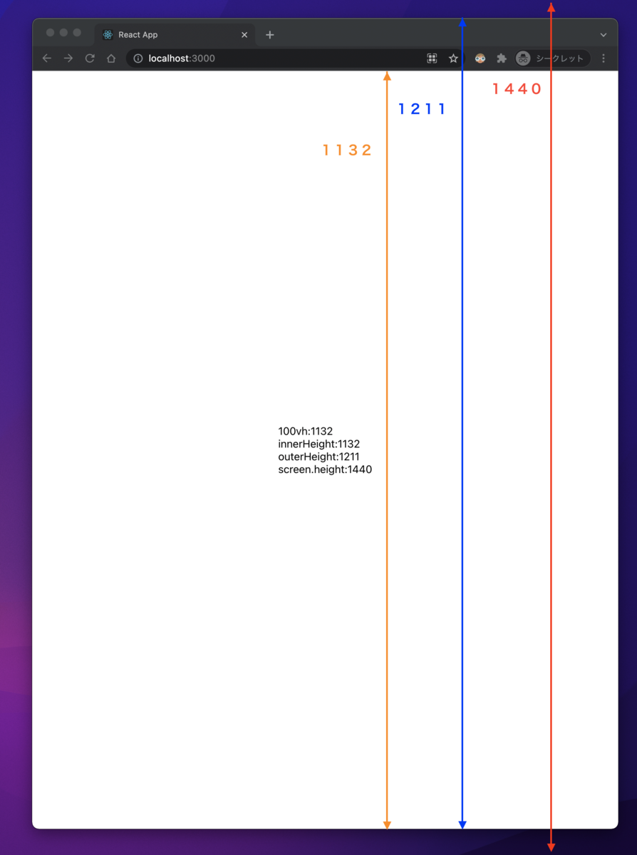 <figcaption>PCブラウザでのvh</figcaption></figure>
innerHeightは、ウィンドウの内部の高さを取得するプロパティで、100vhはこれと同じ値 つまりブラウザ内部の高さいっぱいに広がってくれています。
innerHeight は Window インターフェイスの読み取り専用プロパティで、ウィンドウの内部の高さをピクセル単位で返します。水平スクロールバーがあれば、その高さを含みます。 innerHeight の値はウィンドウのレイアウトビューポート (en-US)の高さから取られます。幅は innerWidth プロパティを使用して取ることができます。 ウィンドウから水平スクロールバーや境界を引いた高さを取得するには、ルートの <html> 要素の clientHeight() プロパティを代わりに使用してください。 Window | innerHeight
スマホでvhの高さを測定する
スマホで100vhを指定した場合、アドレスバーの部分が計算にはいらず、アドレスバー分押し出される形になるので、注意が必要。
アドレスバー分押し出される影響は
-
想定しないスクロールが発生する
-
アドレスバー分、中央配置の要素が少しずれる
対策
CSS変数を使う方法
CSSで-webkit-fill-availableを指定して解決する記事がたくさんありますが、このプロパティは不安定であり、デスクトップ版のChromeで表示が崩れたり、画面サイズに変更があった場合に対応できないという問題があった。
TAKさんの記事では、JavaScriptで高さを計算し、CSS変数を使って対応する方法が書かれています。
CSS変数なので使い回しが簡単という点がイケてる。
JavaScriptで高さを直接指定する
前述したAndroidとiPhoneの例を見ると、100vhを指定した際に、innerHeightの領域外まで広がってしまうのが問題のように感じた。
であれば、画面いっぱいに広げたい要素のラッパーをinnerHeightの高さに合わせて上げれば解決する。
以下は、ReactのuseRefを使った実装例
import {useRef,useCallback,useEffect} from 'react';
import './App.css';

function App() {
  const fullHeightRef = useRef<HTMLDivElement>(null)
   // 画面いっぱいに表示させたい要素にRefを指定

  const setHeight = useCallback(() => {
    if(fullHeightRef.current)  fullHeightRef.current.style.height = `${window.innerHeight}px`
  }, [])

  useEffect(() => {
    setHeight()
    window.addEventListener('resize', setHeight)

    return () => {
      window.removeEventListener('resize', setHeight)
    }
  }, [setHeight])

  return (
    <div className="App" id="App" ref={fullHeightRef}>
      <div className="App__inner">
        画面いっぱいに広げたいコンテンツ
      </div>
    </div>
  );
}

export default App;
とても微妙な調整ではあるが、これがフロントエンドの仕事でもある。 マルチデバイス対応はプロフェッショナルとして意識していきたい。
参考リンク
Reactでモーダルのフォーカス制御の自作にチャレンジした
アクセシビリティを極めていきたい駆け出しフロントエンドエンジニアです。
アクセシビリティな実装をする上で意識すべきことはたくさんありますが、中でもモーダルは考えることが多いなと思っています。
今回は、あえて react-modal などのライブラリを使用せず、自前でアクセシビリティなモーダルを実装してみました。
特に、モーダルを実装する上で肝となる「フォーカス制御」の部分に意識してあります。
アクセシビリティなモーダルとは?
こんなときは、WAI-ARIAのオーサリングプラクティスを参照します。
WAI-ARIAでは、ダイアログ(モーダル)と定義されていますね。
キーボードインタラクションについては以下のようなフローになります。
-
ダイアログが開いたら、フォーカスはダイアログの中に移動
-
タブキーを押したら、次の要素にフォーカスを移動
-
フォーカスがダイアログの中の最後の要素にあれば、ダイアログの中の最初のフォーカス可能要素に移動
-
シフト+タブキーの場合は、前の要素にフォーカスを移動
-
フォーカスがダイアログの中の最初の要素にあれば、ダイアログの中の最後のフォーカス可能要素に移動
-
エスケープキーを押したらダイアログを閉じる
-
ダイアログが閉じられるとき、そのダイアログが呼び出された要素にフォーカスを戻します
言語化するとめちゃくちゃややこしいですが、簡単に言うと「モーダルを開いたらフォーカスを閉じ込める」ということですね。
WAI-ARIAのルール
モーダル関係のWAI-ARIAルールも確認しておきます。
-
ダイアログのコンテナー要素はrole=dialogを持つ
-
ダイアログのコンテナー要素はaria-modalをtrueにセットする
roleを指定することで、スクリーンリーダーで「ダイアログ」と読み上げてくれます。 また、aria-modalをセットすると、ダイアログ以外の要素がアクティブでないことを支援技術に教えてくれるのでで、不要な読み上げが実行されなくなります。
実際にReactでモーダルを作っていく
Reactでアクセシビリティなモーダルコンポーネントを作っていきます。
ここでは、モーダルのコンテンツ部分、CSSスタイリングは割愛しています。
import React, { useState, useCallback, useEffect } from 'react'
import styled from 'styled-components'

const COMPONENT_NAME = 'Modal'

type ModalElement = {
  firstElement: HTMLElement | null
  lastElement: HTMLElement | null
}

type ContainerProps = {
  className?: string
  isMounted: boolean
  modalClose: () => void
}

type Props = {} & ContainerProps

const Component: React.VFC<Props> = ({ isMounted, modalClose, className }) => (
  <>
    {isMounted ? (
      <div className={`${COMPONENT_NAME} ${className}`}>
        <div
          className='dialog'
          id='dialog'
          aria-modal
          role='dialog'
        >
        // Modal Contents
        </div>
      </div>
    ) : null}
  </>
)

const StyledComponent = styled(Component)`
// ...
`

const Container: React.FC<ContainerProps> = (containerProps) => {
  const { isMounted } = containerProps
  const [modalElement, setModalElement] = useState<ModalElement>({
    firstElement: null,
    lastElement: null,
  })

  const handleKeyDown = useCallback(
    (e: KeyboardEvent) => {
      if (e.key === 'Tab') {
        if (e.shiftKey) {
          if (document.activeElement === modalElement.firstElement) {
            modalElement.lastElement?.focus()
            e.preventDefault()
          }
        } else {
          if (document.activeElement === modalElement.lastElement) {
            modalElement.firstElement?.focus()
            e.preventDefault()
          }
        }
      }
    },
    [modalElement.lastElement, modalElement.firstElement]
  )

  useEffect(() => {
    if (isMounted) {
      const focusableEls = document.querySelectorAll(
        '.dialog a[href]:not([disabled]), .dialog button:not([disabled]), .dialog textarea:not([disabled]), .dialog input[type="text"]:not([disabled]), .dialog input[type="radio"]:not([disabled]), .dialog input[type="checkbox"]:not([disabled]), .dialog select:not([disabled])'
      )

      const firstElement = focusableEls[0] as HTMLElement
      const lastElement = focusableEls[focusableEls.length - 1] as HTMLElement

      setModalElement({
        firstElement,
        lastElement,
      })

      firstElement.focus()
      document.addEventListener('keydown', handleKeyDown)
    }

    return () => {
      document.removeEventListener('keydown', handleKeyDown)
    }
  }, [isMounted, handleKeyDown])

  return <StyledComponent {...containerProps} />
}

export default Container
Containerコンポーネントの部分で、フォーカスの制御を行っています。
モーダル内にフォーカスを制御させる
  const handleKeyDown = useCallback(
    (e: KeyboardEvent) => {
      if (e.key === 'Escape') {
        modalClose()
      }
      if (e.key === 'Tab') {
        if (e.shiftKey) {
          if (document.activeElement === modalElement.firstElement) {
            modalElement.lastElement?.focus()
            e.preventDefault()
          }
        } else {
          if (document.activeElement === modalElement.lastElement) {
            modalElement.firstElement?.focus()
            e.preventDefault()
          }
        }
      }
    },
    [modalElement.lastElement, modalElement.firstElement, modalClose]
  )
-
タブキーでの移動またはタブ+シフトキーでの移動
-
document.activeElementで現在フォーカスがあたっている要素を取得 -
モーダル内の最初又は最後のフォーカス可能要素がアクティブだった場合、最初又は最後の要素にフォーカスを移す。
-
ESCキーが押されたら、モーダルを閉じる
フォーカスしている要素とモーダル内のフォーカス可能な子要素をチェックして、モーダル内でのフォーカス制御を実現できました。
参考にしたのはこちらの記事
  useEffect(() => {
    if (isMounted) {
      const focusableEls = document.querySelectorAll(
        '.dialog a[href]:not([disabled]), .dialog button:not([disabled]), .dialog textarea:not([disabled]), .dialog input[type="text"]:not([disabled]), .dialog input[type="radio"]:not([disabled]), .dialog input[type="checkbox"]:not([disabled]), .dialog select:not([disabled])'
      )

      const firstElement = focusableEls[0] as HTMLElement
      const lastElement = focusableEls[focusableEls.length - 1] as HTMLElement

      setModalElement({
        firstElement,
        lastElement,
      })

      firstElement.focus()
      document.addEventListener('keydown', handleKeyDown)
    }

    return () => {
      document.removeEventListener('keydown', handleKeyDown)
    }
  }, [isMounted, handleKeyDown])
ここで行っているのは、マウント時にフォーカス可能要素を取得してフォーカスを当てる処理と、イベントリスナーの設定です。
-
モーダルがマウントされたとき、モーダル内のフォーカス可能要素を取得
-
そのうち最初と最後の要素をStateに格納
-
最初の要素にフォーカスを当てる
-
keydownイベントでhandleKeyDown関数を発火させる
-
アンマウント時にイベントリスナーを削除
モーダルを閉じたときにフォーカスを元に戻す
最後に、モーダルを閉じたときにフォーカスを元のページに戻す処理です。
便利なuseRefを使い、モーダルを閉じた際にフォーカスを元に戻す処理を書いているだけです。
  const modalButtonRef = useRef<HTMLButtonElement | null>(null)

  const modalClose = useCallback(() => {
    setIsMounted(false)
    modalButtonRef.current?.focus()
  }, [setIsMounted])
モーダルを開くトリガーになっているボタンにフォーカスを戻すのが通常のようですので、今回はボタンにrefを設定しました。
        <button type='button' onClick={modalOpen} ref={modalButtonRef}>
          モーダルを開く
        </button>
動作確認
さて、これで問題無さそうか動作確認してみます。
モーダルを展開した後、フォーカスがモーダル内に制御されます。
ESCキーでモーダルを閉じた後は、「モーダルを開く」ボタンにフォーカスが戻っていて、ユーザーが困惑することも無さそうです。
ここまで自作でフォーカス制御を実装してきましたが、focus-trap-reactを使うと簡単に実装できます。
アクセシビリティの深みへ
単純にデザインを実装するだけではなく、アクセシビリティを追求して細かいUIを作っていくのは興味深いです。
とはいえ、本日実装したものでは不十分な部分もあるかもしれないので、まだまだアクセシビリティに関する知見は吸収しつつアウトプットしていきたいですね。
アクセシビリティ対策をすることになったので、a11yについてまとめてみた
アクセシビリティとは
アクセシビリティの言葉のとおり、アクセスのしやすさを意味していて、コンテンツの利用がしやすさとほぼ同義だとおもいます。
ユーザービリティは使いやすさ アクセシビリティは、更に幅広い人や状況でも使えることという棲み分けでしょうか。
それがウェブになるとどうなるか。 ウェブコンテンツは、様々なユーザーがそれぞれ異なるデバイスを使ってアクセスし、かつ使用している状況も様々です。
アクセシビリティと言うと、「身体的な障害を持った人のもの」というイメージがつきまといますが、誰かのための特別な対応ではなく、すべての人に向けた普遍的な対応を指します。 身体的な障害を持つ方だけでなく、さまざまな環境・状況にいる方、高齢者なども含んだ考え方です。
すべての人に向けた普遍的な対応ってすごく良い。頑張って作ったサービスだからこそ、一人も不自由なく使ってほしい、私もそう思い、アクセシビリティの勉強をはじめました。
例えば、、、
以下の様に身体の障害がある方はもちろんですが、高齢による状態の変化や一時的な障害があったとしてもコンテンツが利用できることが目指すべき状態だと考えます。
-
身体の障害
-
一時的な障害
-
コンタクト紛失・メガネが壊れた → 画面拡大
-
手の骨折、利き手が使えない状況 → キーボード操作
-
マウスが壊れた、マウスが使えない・使いづらい状況 → キーボード操作
-
アクセシビリティの規格
現在、国内規格のJIS、W3Cの勧告、国際規格のISOが完全に統一されています
-
JIS X 8341-3:2016
-
WCAG 2.0
-
ISO/IEC 40500:2012
ウェブコンテンツのアクセシビリティ
ウェブアクセシビリティに関しては、W3Cが出しているWCAG(ウェブコンテンツアクセシビリティ)が参考になります。
ウェブ・コンテンツ・アクセシビリティ・ガイドライン(WCAG)2.0WCAG 2.0 解説書WCAG 2.0 達成方法集
ウェブアクセシビリティ基盤委員会にはウェブアクセシビリティ方針策定ガイドラインが作成されていますが、多くの起業でアクセシビリティガイドラインが作成・公開されており、非常にわかりやすいものが多いのでこれらを流用している起業も増えてきている印象です。
実際に私が勤務している起業でも、freee のアクセシビリティガイドラインをそのまま使用することにしました。
WCAGの基準はどこまでを目指すか?
WCAGの基準は適合レベルが設けられており、レベルが3段階ある。
-
レベルA
-
レベルAA
-
レベルAAA → 最高レベル
いきなり最高レベルを目指すのはかなりハードルが高いので、まずはA基準を満たしつつ、徐々にレベルを挙げていくのが良さそう。
プロダクトによっては、レベルAを基準にしつつも、レベルAAの基準も満たせるものが出てくるので追加して対応していってもいいかと思う。
WAI_ARIAの対応は必要なのか?
HTMLで表現できる範囲を逸脱したUIを作る時はWAI-ARIA対応が必要という認識を持っている。 基本的には、セマンティックなマークアップを行っていればAria属性は付ける必要はないが、 <div>でマークアップした要素でゴリゴリカスタマイズしたりする場合は、 aria属性をつけて上げる必要がある。
WAI-ARIAはスクリーンリーダー対応をするにあたって重要な役割を担う。
「どのような場面でWAI-ARIAを使うのか?」についてはHTMLで表現できる範囲を逸脱したUIを作る時だと思っている。
-
ランドマーク ariaの
role属性はランドマークになる -
動的なコンテンツの更新(コンテンツが更新されたときにスクリーンリーダーで伝える)
-
キーボードのアクセシビリティ向上(TabIndex)
-
<div>のネストなど複雑なUIを構築する場合
「もう一度言いますが、必要な時だけ使ってください!」 MDNでも繰り返し言われているので、必要な場合のみ使うようにする。
ベストプラクティスは、WAI-ARIAオーサリング・プラクティスで確認する。
アクセシビリティはやればやるほど良い
どこかのカンファレンスで話されていたことが印象的で覚えているのですが、「アクセシビリティはやらなければマイナスというわけではなく、やればやるほどプラスになる加点方式だ」ということ。
やればやるほどプロダクトの質が上がるなら、やらない理由は無いなと個人的には思うわけです。
ただ、どこまで工数を割いていいかは相談しながら。
関連リンク
ReactのErrorBoundaryとは何か
ErrorBoundary
コンポーネントツリーのどこかで例外が発生した場合、アプリケーション全体が影響を受けてしまう。アプリの規模が大きくなると、例外が発生した箇所を特定するのが難しくなってくる。
ErrorBoundaryは、特定のコンポーネントで例外が発生したとしても、アプリ全体に影響を与えずフォールバック用の UI を表示するコンポーネント。
ErrorBoundaryコンポーネントの作成
ErrorBoundaryを実装するには、ライフサイクルメソッドの getDerivedStateFromError か、 componentDidCatch を使う必要がある。つまり、関数コンポーネントでのErrorBoundaryはできず、クラスコンポーネントを実装しないといけないみたい。
ErrorBoundary.tsx
import React, { ErrorInfo } from "react";

class ErrorBoundary extends React.Component<{}, { hasError: boolean }> {
  constructor(props: {}) {
    super(props);
    this.state = {
      hasError: false
    };
  }

  static getDerivedStateFromError(): { hasError: boolean } {
    console.log("getDerivedStatefromError");
    return { hasError: true };
  }

  componentDidCatch(error: Error, errorInfo: ErrorInfo): void {
    console.log("this.state.hasError", this.state.hasError);
    console.log(error);
    console.log(errorInfo);
  }

  render() {
    if (this.state.hasError) {
      console.log("render", this.state.hasError);
      return <>エラーが発生したよ!</>;
    }
    return <>{this.props.children}</>;
  }
}

export default ErrorBoundary;
ほぼ公式ドキュメントからの抜粋 error boundaryとは
-
getDerivedStateFromError()... 名前のとおり、エラーをキャッチしてstateを更新するためのオブジェクト。更新するstate情報をreturnすることでsetState()される。 -
componentDidCatch()... エラー情報をキャッチする。ErrorとErrorInfo
該当コンポーネントをErrorBoundaryコンポーネントで囲む
エラーを発生させるコンポーネントを作成。
BreakThings.tsx
export const BreakThings = () => {
  throw new Error("Something went wrong!");
};
App.tsx
import "./styles.css";
import SiteLayout from "./SiteLayout";
import ErrorBoundary from "./ErrorBoundary";
import { BreakThings } from "./BreakThings";

export default function App() {
  return (
    <div className="App">
      <SiteLayout
        menu={
          <ErrorBoundary>
            <BreakThings />
            <p>Menu</p>
          </ErrorBoundary>
        }
      >
        <>
          <h1>Heading</h1>
        </>
      </SiteLayout>
    </div>
  );
}
単一のコンポーネントをラップすると、それぞれでエラーが発生した場合、個別にfallbackコンポーネントが表示されます。
ただし、開発用サーバーだとスタックトレース情報が表示されてしまうので、アプリケーションをビルドした上で確認したほうが良さそう。
関数型で扱えるパッケージreact-error-boundary
react-error-boundaryを使用すれば、レンダリング時のエラーが扱いやすくなるみたい。
import {ErrorBoundary} from 'react-error-boundary'

function ErrorFallback({error, resetErrorBoundary}) {
  return (
    <div role="alert">
      <p>Something went wrong:</p>
      <pre>{error.message}</pre>
      <button onClick={resetErrorBoundary}>Try again</button>
    </div>
  )
}

const ui = (
  <ErrorBoundary
    FallbackComponent={ErrorFallback}
    onReset={() => {
      // reset the state of your app so the error doesn't happen again
    }}
  >
    <ComponentThatMayError />
  </ErrorBoundary>
)****
ドキュメントからの抜粋ですが、やはり関数型の方がシンプルで良き。
関連リンク
ReactHooksについてのまとめ
Hooksとは?
React16.8.0で追加された機能
-
クラスコンポーネントよりもコード量が少なくなる
-
ロジックを分離できるので、ロジックの再利用やテストがしやすい。
主なフックとしてあげられているものをまとめてみる
useState
stateと、state更新関数を返すフック
このフックを利用すれば、コンポーネント内でstate管理ができる
useStateは戻り値として、state変数とstate更新関数をタプルとして返すので、分割代入で受け取る
import { useState } from "react";

export default function App() {
const [count, setCount] = useState<number>(0);

  const onClickSetCount = () => {
    setCount(count + 1);
  };
  return (
    <div className="App">
      <p>{count}</p>
      <button onClick={onClickSetCount}>add</button>
    </div>
  );
}
ちなみに「state」とは、画面に表示されるデータやUIの状態など、アプリケーションが保持している情報(データや値)のこと
また、「state管理」とは、stateの保持とstateの更新をすることを指す
注意:レンダリングごとに state 変数は一定
const plusThreeDirectly = () =>
		[0, 1, 2].forEach((_) => setCount(count + 1));
// 1

const plusThreeWithFunction = () =>
    [0, 1, 2].forEach((_) => setCount((c) => c + 1));
// 3
この挙動の違い
state 変数はそのコンポーネントのレンダリングごとで一定
plusThreeDirectly() はそのレンダリング時点での count が 0 だったら、それを 1 に上書きする処理を 3 回繰り返すことになる
state 変数を相対的に変更する処理を行うときは、
前の値を直接参照・変更するのは避け、必ず setCount((c) => c + 1) のように関数で書くこと。
クラスコンポーネントでは this.state には常に最新の値が入ってるのに対し、State Hook ではレンダリングごとに state 変数は一定というちがいがあるの
注意:呼び出しはその関数コンポーネントの論理階層のトップレベル
条件文や繰り返し処理の中で呼びだすのはタブー
const Counter: VFC<{ max: number }> = ({ max }) => {
  const [count, setCount] = useState(0);

  if (count >= max) {
    const [isExceeded, setIsExceeded] = useState(true);
    doSomething(...);
  }
TypeScriptでuseStateを使う際の注意
■stateの型が推論できるかどうか
外部APIから値を取得し、Stateに入れる場合だと、初期値として渡せる型を持ったデータがない。
そういうときは型推論に任せず、useState に明示的に型引数を渡してあげる必要がある
const [author, setAuthor] = useState<User>();
Userオブジェクト型を型引数として渡し、useStateの引数には何も渡していない
→ author は User オブジェクトを格納でき、初期値が undefined の変数になる。
undefined ではなく、明示的に null を入れたい場合はこうする
useState<User | null>(null)
引数に [] だけをわたすとなんの配列かわからないので、 useState<Article[]>([]); とする
オブジェクト配列の場合(TypeScript)
import {useState } from "react";
interface Todo {
  id: number;
  title: string;
  complete: boolean;
}

const data = [
  {
    id: 1,
    title: "todo1",
    complete: true
  },
  {
    id: 2,
    title: "todo2",
    complete: false
  },
  {
    id: 3,
    title: "todo3",
    complete: false
  }
];

export default function Todos() {
  const [todos, setTodos] = useState<Array<Todo>>(data);

  // const [todos, setTodos] = useState<Todo[]>(data);
<Array<Todo>> は <Todo[]> と同義
[ { } ] の形をあらわす。
オブジェクトのプロパティ型を定義するには interface を使う
interface Todo {
  id: number;
  title: string;
  complete: boolean;
}
useEffect
副作用って?英語では side-effect
→ コンポーネントの状態を変化させて、それ以降の出力を変えてしまうこと
コンポーネントがレンダーされるたびに副作用を実行
useEffect(() => {
	console.log('component render')
})
コンポーネントがレンダーされたときに1度だけ実行
useEffect(() => {
	console.log('component render')
},[])
副作用に依存する配列が更新したときだけ実行
useEffect(() => {
	 console.log(count)
},[count])
副作用内で関数をreturnすると、その関数はコンポーネントがアンマウントもしくは副作用が再実行されたときに実行される。
ライフサイクルメソッドでいうとそれぞれ以下に対応している
-
useEffectの第2引数に空配列を渡す ...componentDidMount -
何も渡さない ...
componentDidUpdate
メモ化
関数コンポーネントの中に、計算リソースを多大に消費する処理が内包されていたとして、結果が同じなのにレンダリングのたびに再計算されるのを防ぐ
パフォーマンス最適化のために、必要なときだけ計算し、「メモ’
コンポーネントが再レンダリングされたら、関数も再定義されてしまう。
それを防ぐために useCallback と useMemoを使う
依存配列にpropsを指定すれば、props が変わったときだけ、関数の再定義が行われるようになり、不要な再レンダリングを防ぐことができる。
useCallback
関数定義そのものをメモ化する
const reset = useCallback(() => setTimeLeft(limit), [limit]);
useMemo
関数の実行結果をメモ化する
const primes = useMemo(() => getPrimes(limit), [limit]);
useRef
refオブジェクトを生成するHooks
-
初回のレンダリング時にテキストフォームにフォーカス
-
onClickによってフォームの入力値を取得
import { useEffect, useState, useCallback, useRef } from "react";

const refInput = useRef();

useEffect(() => {
    console.log(refInput.current);
    // => <input value="refInput."></input>

    refInput.current.focus();
  }, []);

return (
	<input onChange={onChangeText} value={text} ref={refInput} />
)
あらゆる書き換え可能な値を保持しておくことができる
const timerId = useRef();

useEffect(()=>{
  timerId.current = setInterval(60,1000)

  return () => clearInterval(timerId.current)
},[])
useRef で最新のタイマーIDを保持するようにできる
useRefはuseStateと違い、値の変更がコンポーネントの再レンダリングを発生させないのがポイント
useReducer
複雑なState更新時のsetter関数として
**import React, { useState, useReducer } from 'react';

export default function App() {
  const data = {
    id: 1,
    name: 'hobehobe',
    phone: '03-0000-1111',
    email: 'mail@example.com',
    admin: false
  };
  // const [user, setUser] = useState(data);

  const [user, setUser] = useReducer(
    (user, newDetails) => ({ ...user, ...newDetails }), // dispatch
    data // initial state
  );

  const handleClick = () => {
    // useStateだと、スプレッド構文で展開する必要がある
    // setUser({ ...user, admin: true });
    setUser({ admin: true });

    /*
    変更部分のみ更新される
    admin: true
    email: "mail@example.com"
    id: 1
    name: "hobehobe"
    phone: "03-0000-1111"
    */
  };

  console.log(user);
  return (
    <>
      <button onClick={handleClick}>click</button>
    </>
  );
}**
useContext と組み合わせて、reduxっぽく使う
immer
useContext
useReducer
npm install use-immer immerimport React, { useEffect, useState, useReducer } from "react";
import { useImmerReducer } from "use-immer";
import StateContext from "./StateContext";
import DispatchContext from "./DispatchContext";
const App = () => {
// stateの初期値を定義
const initialState = {
loggedIn: Boolean(localStorage.getItem("complexappToken")),
flashMessages: [],
user: {
// 初期値はローカルストレージから取得
token: localStorage.getItem("complexappToken"),
username: localStorage.getItem("complexappUsername"),
avatar: localStorage.getItem("complexappAvatar"),
},
};
/*
immerを使って、recuderを定義
毎回オブジェクト全体をreducer で定義する必要がなくなる。
変更部分のみ、処理するだけでいい
*/
const ourReducer = (draft, action) => {
switch (action.type) {
case "login":
draft.loggedIn = true;
draft.user = action.data;
return;
case "logout":
draft.loggedIn = false;
return;
case "flashMessage":
draft.flashMessages.push(action.value);
return;
}
};
// reducer と state初期値
const [state, dispatch] = useImmerReducer(ourReducer, initialState);
return(
<StateContext.Provider value={state}>
<DispatchContext.Provider value={dispatch}>
<Component />
</DispatchContext.Provider>
</StateContext.Provider>
)
}
DicpatchContext.js
import { createContext } from "react";

const DispatchContext = createContext();

export default DispatchContext;
StateContext.js
import { createContext } from "react";

const StateContext = createContext();

export default StateContext;コンポーネントでstateとdispatchにアクセスする
import React, { useContext } from "react";
import DispatchContext from "../DispatchContext";
import StateContext from "../StateContext";

const Component = () => {
const appDispatch = useContext(DispatchContext);
const appState = useContext(StateContext);

  const handleLogout = () => {
    appDispatch({ type: "logout" });
  };

}
素のアクションオブジェクトをdispatchしているが、
action creatorを作成したほうがよさそう
useContext
provider を作る
管理するStateごとに作る。
import { createContext, useState } from "react";

export const UserContext = createContext({});

export const UserProvider = (props) => {
  const { children } = props;

// stateを定義
  const [userInfo, setUserInfo] = useState(null);

// Providerのvalueに渡
  return (
    <UserContext.Provider value={{ userInfo, setUserInfo }}>
      {children}
    </UserContext.Provider>
  );
};
App.js でStateを使いたいタグをラップする (ここでは全体)
import React, { UserProvider } from "./providers/UserProvider";
import { Router } from "./router/Router";
import "./styles.css";

export default function App() {
  return (
    <UserProvider>
      <Router />
    </UserProvider>
  );
}コンポーネント側で使用
import React, { useContext } from "react";
import { UserContext } from "../../../providers/UserProvider";

export const UserIconWithName = (props) => {

	const { userInfo } = useContext(UserContext);

	const isAdmin = userInfo ? userInfo.isAdmin : false;

	const { setUserInfo } = useContext(UserContext);

	const onClickAdmin = () => {
	    setUserInfo({ isAdmin: true });
	  };
再レンダリングの注意点
1つのプロバイダの中で渡している値(ここでは userInfo, setUserInfo )が 使われているコンポーネントが再レンダリングされてしまうので注意が必要。
更新時に「どのコンポーネントが再レンダリングされるか?」を意識しながら開発する必要がある。
子コンポーネントを memo 化 など、再レンダリングの最適化を行う必要がある
参考
カスタムフック
src/hooks/useAllUsers.ts
import axios from "axios";
import { useState } from "react";
import { userProfile } from "../types/userProfile";
import { User } from "../types/api/user";

// 全ユーザー一覧を取得するカスタムフック
export const useAllUsers = () => {
  const [userProfiles, setUserProfile] = useState<Array<userProfile>>([]);
  const [loading, setLoading] = useState(false);
  const [error, setError] = useState(false);

  const getUsers = () => {
    setLoading(true);
    setError(false);

    axios
      .get<Array<User>>("<https://jsonplaceholder.typicode.com/users>")
      .then((res) => {
        const data = res.data.map((user) => ({
          id: user.id,
          name: `${user.name}(${user.username})`,
          email: user.email,
          address: `${user.address.city}${user.address.suite}${user.address.street}`
        }));
        setUserProfile(data);
      })
      .catch(() => {
        setError(true);
      })
      .finally(() => {
        setLoading(false);
      });
  };

  return {
    getUsers,
    userProfiles,
    loading,
    error
  };
};コンポーネント側から利用
App.tsx
import { useAllUsers } from "./hooks/useAllUsers";

const { getUsers, userProfiles, loading, error } = useAllUsers();

const onClickFetchUser = () => getUsers();
useStateなどと同じように使用するだけで、簡単に実行できる。
関連リンク
カスタムフックは再利用できるため公開されているものを利用することもできる
Zodで基本的なバリデーションをかけてみる
バリデーションライブラリ「Zod」の基本的な使い方についてまとめてみる。
Zodは、スキーマファーストなバリデーションライブラリ。 はじめにスキーマを定義して、パースすることでバリデーションをかけることができる。
スキーマを定義する
varidation.ts
import { z } from "zod";

export type ValidationErrors = { [k: string]: string[] };

// schemaの定義
export const schema = z.object({
  text: z
    .string()
    .nonempty({ message: "入力は必須です。" })
    .min(5, "5文字以上で入力してください。")
});

export type TextInput = z.infer<typeof schema>;

// バリデーションに成功したら、データを返す
// 失敗すれば、エラーメッセージを返す
export const textValidate = (
  targetData: TextInput,
  success?: (result: TextInput) => void,
  fail?: (errors: ValidationErrors) => void
): void => {
  const result = schema.safeParse(targetData);

  if (result.success) {
    if (success) success(result.data);
  } else if (fail) fail(result.error.flatten().fieldErrors);
};
nonemptyは入力必須 minは最小文字数を定義できる 続けて、表示したいエラーメッセージを記述することができる。 上記のバリデーションを実行して、エラーメッセージを格納するロジックをカスタムフックに分離させる。
エラーメッセージを取得して格納する
hooks.ts
import { useCallback, useState } from "react";
import { textValidate, TextInput, ValidationErrors } from "./varidation";

export const useValidation = (): {
  validateErrors: ValidationErrors;
  doValidate: (textInput: TextInput, cb?: (result: TextInput) => void) => void;
} => {
// エラーメッセージの格納
  const [validateErrors, setValidateErrors] = useState<ValidationErrors>({
    text: []
  });

  const doValidate = useCallback(
    (textInput: TextInput, cb?: (result: TextInput) => void) => {
      textValidate(
        textInput,
        (result: TextInput) => {
          setValidateErrors({
            text: []
          });
          if (cb) cb(result);
        },
        (errors) => {
          setValidateErrors({
            ...errors
          });
        }
      );
    },
    []
  );

  return { validateErrors, doValidate };
};
エラーメッセージは、複数のフォームに対応するため、オブジェクトで持たせる
{
    email: []
		password: []
}
コンポーネントで使用
App.tsx
import React, { useState, useCallback } from "react";
import styled from "styled-components";
import { useValidation } from "./hooks";
import { TextInput } from "./varidation";
import TextInputField from "./TextInput";
import InputError from "./InputError";

import "./styles.css";

export type Props = {
  className?: string;
};

export const App: React.VFC<Props> = ({ className }) => {
  const [Input, setInput] = useState({ text: "" });
  const { validateErrors, doValidate } = useValidation();

  const changeInput = useCallback(
    (e: React.ChangeEvent<HTMLInputElement>) => {
      setInput({
        text: e.target.value
      });
    },
    [setInput]
  );

  const handleSubmit = (e: React.FormEvent) => {
    e.preventDefault();
    doValidate(Input, (result: TextInput) => console.log(result));
  };

  return (
    <div className={className}>
      <form onSubmit={handleSubmit}>
        <div className={`formInput`}>
          <InputError errorMessages={validateErrors.text}>
            <TextInputField
              name="text"
              placeholder="Text"
              onChange={changeInput}
              value={Input.text}
              isError={validateErrors.text.length > 0}
            />
          </InputError>
        </div>
        <button type="submit">Submit</button>
      </form>
    </div>
  );
};

export const StyledComponent = styled(App)`
  padding: 16px;

  form {
    margin: 0 auto;
  }
`;

export default StyledComponent;
設定したバリデーションエラーを格納して、エラーメッセージを表示することができた。 <InputError>コンポーネントは、単純にエラーメッセージを受け取って、表示するだけのコンポーネント。