【scikit-learn】パーセプトロンでアヤメの分類を実装
今回は、パーセプトロンでアヤメの分類を実装していきたいと思います。
パーセプトロンとは
分類問題に使われる手法の一つで、いわゆる「教師あり学習」を行うためのもの。
「あるデータがどのグループに属するか」を学習して、未知のデータからグループごとに分類することができる。
「教師ラベル」といって、学習用データにはどのグループに属しているかという情報があらかじめ与えられていて、この「教師データ」を使って学習していきます。
パーセプトロンは、実はあまり使われていないらしく その理由としては
「与えられたデータが線形分離可能でなければアルゴリズムが収束しない」 という弱点があるかららしい。
線形分離とは、その名前の通りで「一本の直線で二つのグループに分離できる」ことです。 複雑な分類には向いていないのかなーと。
scikit-learnのirisデータセットを使って分類してみました。
アヤメのサンプルデータの準備
# import
import pandas as pd
import numpy as np
from matplotlib import pyplot as plt
%matplotlib inline
import seaborn as sns

# import datasets
from sklearn import datasets
iris = datasets.load_iris()
X = iris.data[:,[2,3]]
y = iris.target

# データセット分割 テストデータ30%
from sklearn.model_selection import train_test_split

X_train,X_test,y_train,y_test = train_test_split(X,y,test_size=0.3,random_state=1,stratify=y)
データの標準化
from sklearn.preprocessing import StandardScaler
sc = StandardScaler()

# トレーニングデータの平均と標準偏差を計算
sc.fit(X_train)

#平均と標準偏差を用いて標準化
X_train_std = sc.transform(X_train)
X_test_std = sc.transform(X_test)
トレーニングデータとテストデータの値を相互に比較できるように、標準化をしておく
パーセプトロンのインポート、学習
# パーセプトロンのインポート
from sklearn.linear_model import Perceptron
# エポック数40、学習率0.1でパーセプトロンのインスタンス作成
ppn = Perceptron(eta0=0.1, random_state=1)
# トレーニングデータをモデルに適合
ppn.fit(X_train_std, y_train)

# 予測
y_pred = ppn.predict(X_test_std)
accuracy_scoreで正解率を確認してみます。
# 分類の正解率
from sklearn.metrics import accuracy_score

print('Accuracy: %.2f' % accuracy_score(y_test, y_pred))
# print('Accuracy: %.2f' % ppn.score(X_test_std, y_test)) score でもOK
Accuracy: 0.98 0.98?精度高すぎませんか?
決定領域をプロット
from matplotlib.colors import ListedColormap
def plot_decision_regions(X,y,classifier, test_idx=None,resolution=0.02):

   # マーカーとカラーマップ
   markers = ('s','x','o','^','v')
   colors = ('red','blue','lightgreen','gray','cyan')
   cmap = ListedColormap(colors[:len(np.unique(y))])

   # 決定領域のプロット
   x1_min, x1_max = X[:,0].min() - 1, X[:,0].max() + 1
   x2_min, x2_max = X[:,1].min() - 1, X[:,1].max() + 1

   # グリッドポイントの生成
   xx1,xx2 = np.meshgrid(np.arange(x1_min,x1_max,resolution),
                        np.arange(x2_min,x2_max,resolution))

   # 各特徴量を1次元配列に変換して予測を実行
   Z = classifier.predict(np.array([xx1.ravel(), xx2.ravel()]).T)

   # 予測結果を元のグリッドポイントのデータサイズに変換
   Z = Z.reshape(xx1.shape)

   # グリッドポイントの等高線のプロット
   plt.contourf(xx1,xx2,Z,alpha=0.3,cmap=cmap)

   # 軸の範囲の設定
   plt.xlim(xx1.min(), xx1.max())
   plt.ylim(xx2.min(), xx2.max())

   # クラスごとにサンプルをプロットする
   for idx, cl in enumerate(np.unique(y)):
       plt.scatter(x=X[y == cl, 0], y=X[y == cl,1],
                  alpha=0.8,
                  c=colors[idx],
                  marker=markers[idx],
                  label=cl,
                  edgecolor='black')

   # テストサンプルを目出させる
   if test_idx:
       X_test, y_test = X[test_idx, :], y[test_idx]
       plt.scatter(X_test[:,0], X_test[:,1],
                  c='',
                  edgecolor='black',
                  alpha=1.0,
                  linewidth=1,
                  marker='o',
                  s=100,
                  label='test set')


# トレーニングデータとテストデータの特徴量を行方向に結合
X_combined_std = np.vstack((X_train_std, X_test_std))

# トレーニングデータとテストデータのクラスラベルを結合
y_combined = np.hstack((y_train,y_test))

# 決定領域のプロット
plot_decision_regions(X=X_combined_std, y=y_combined, classifier=ppn,
                    test_idx=range(105,150))

plt.xlabel('petal length [std]')
plt.ylabel('petal width [std]')

plt.legend(loc='upper left')

plt.tight_layout()
plt.show()
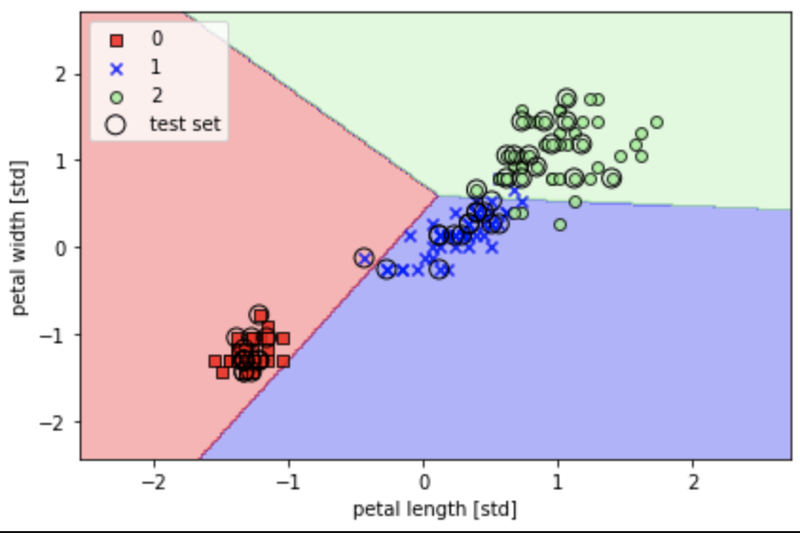
正解率は高かったですが、、
「3つの品種(多クラス)を線形の決定境界で完全に区切ることはできない」ということがわかりました。
今回はこのくらいにして、次回からはロジスティック回帰や決定木で分類してみたいと思います。